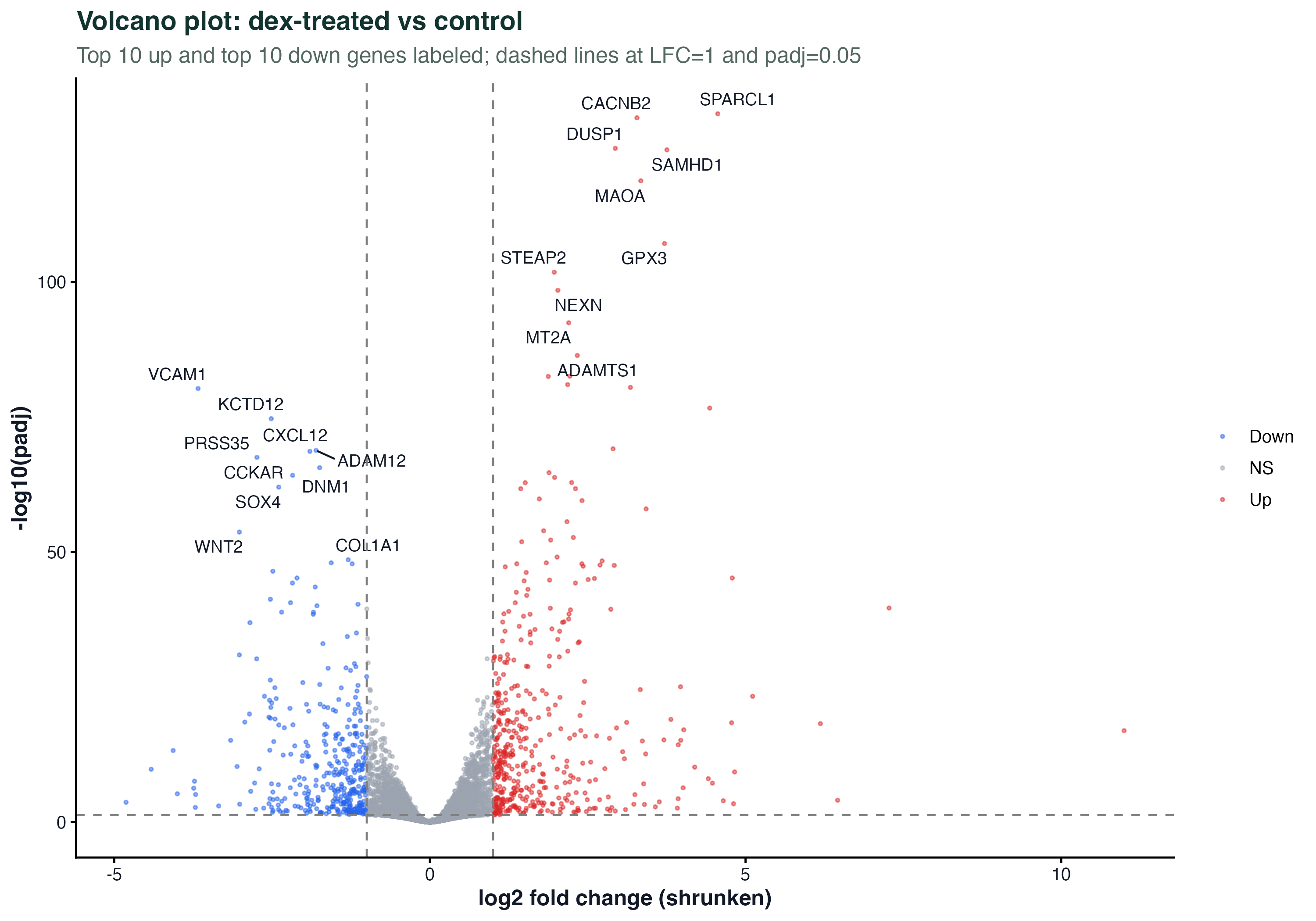
Volcano Plot
ggplot(de_df, aes(x = log2FC, y = -log10(padj), color = sig)) +
  geom_point(size = 0.6, alpha = 0.5) +
  geom_text_repel(data = top, aes(label = symbol), size = 3) +
  scale_color_manual(values = c(Up="#dc2626", Down="#2563eb", NS="#9ca3af")) +
  geom_vline(xintercept = c(-1, 1), linetype = "dashed") +
  geom_hline(yintercept = -log10(0.05), linetype = "dashed") +
  theme_classic()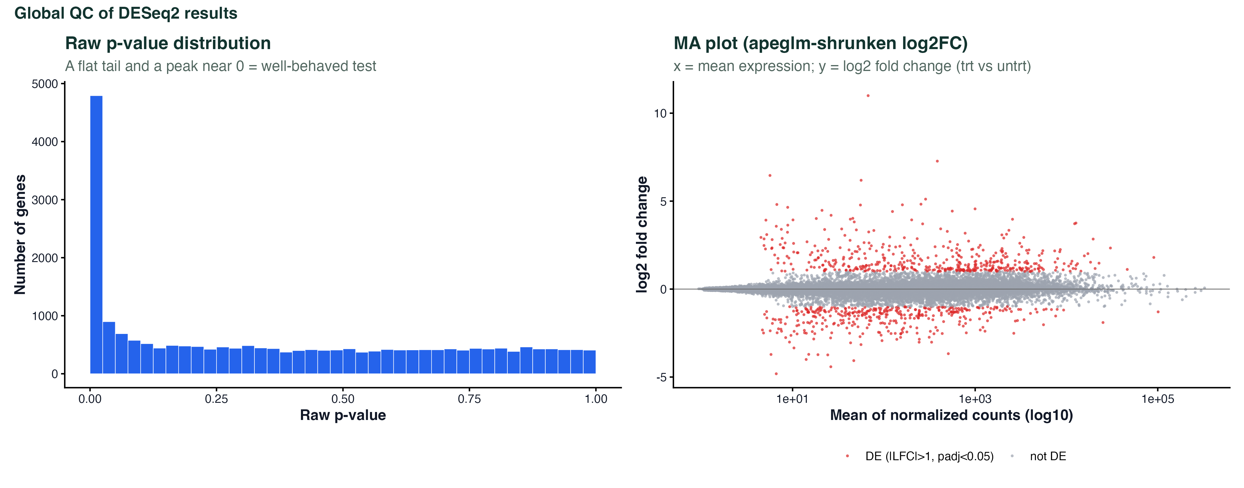
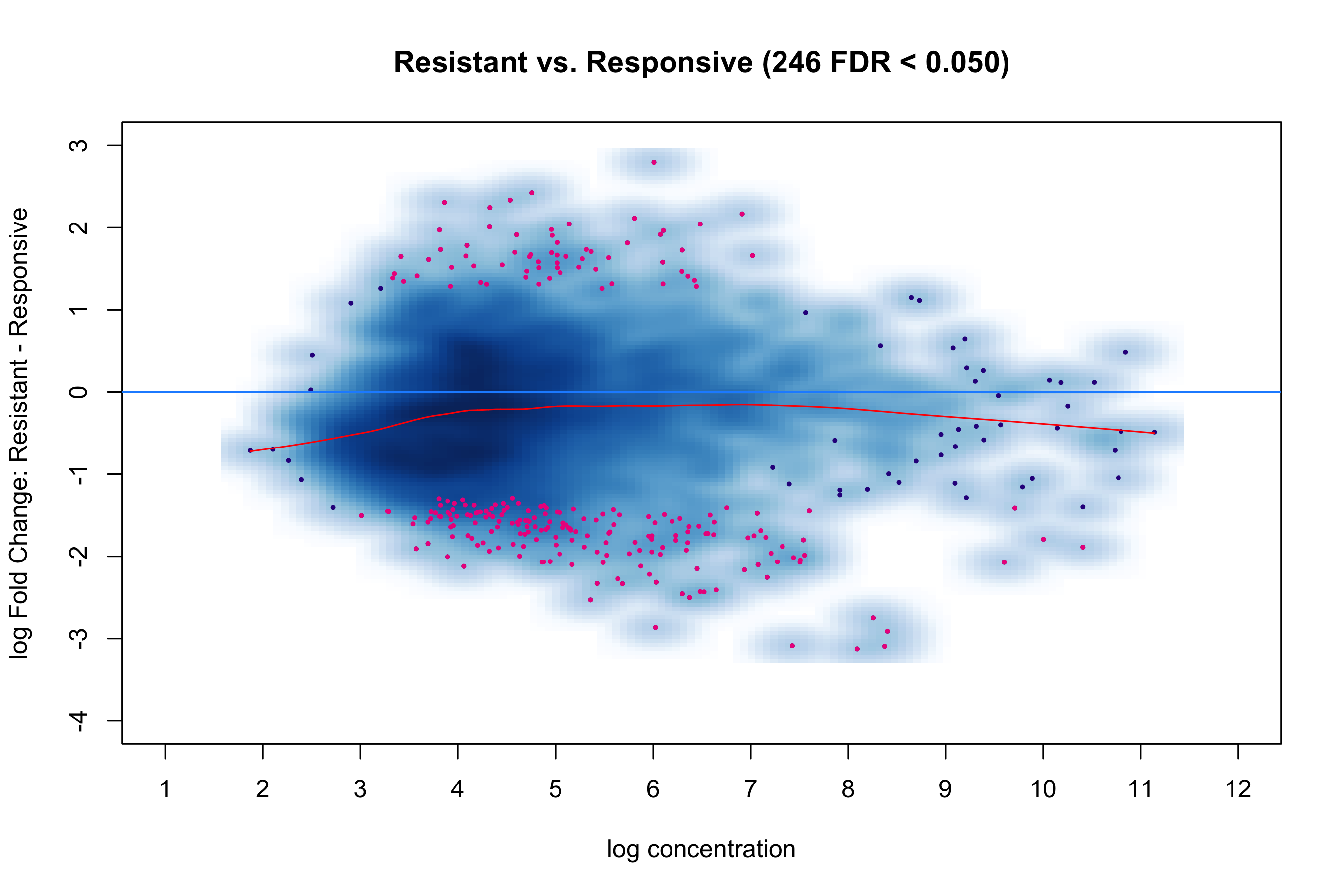
MA Plot
ggplot(ma_df, aes(x = baseMean, y = log2FC, color = sig)) +
  geom_point(size = 0.4, alpha = 0.5) +
  scale_x_log10() +
  scale_color_manual(values = c(DE="#dc2626", NS="#9ca3af")) +
  geom_hline(yintercept = 0, color = "grey40") +
  labs(x = "Mean expression (log10)", y = "log2 Fold Change") +
  theme_classic()
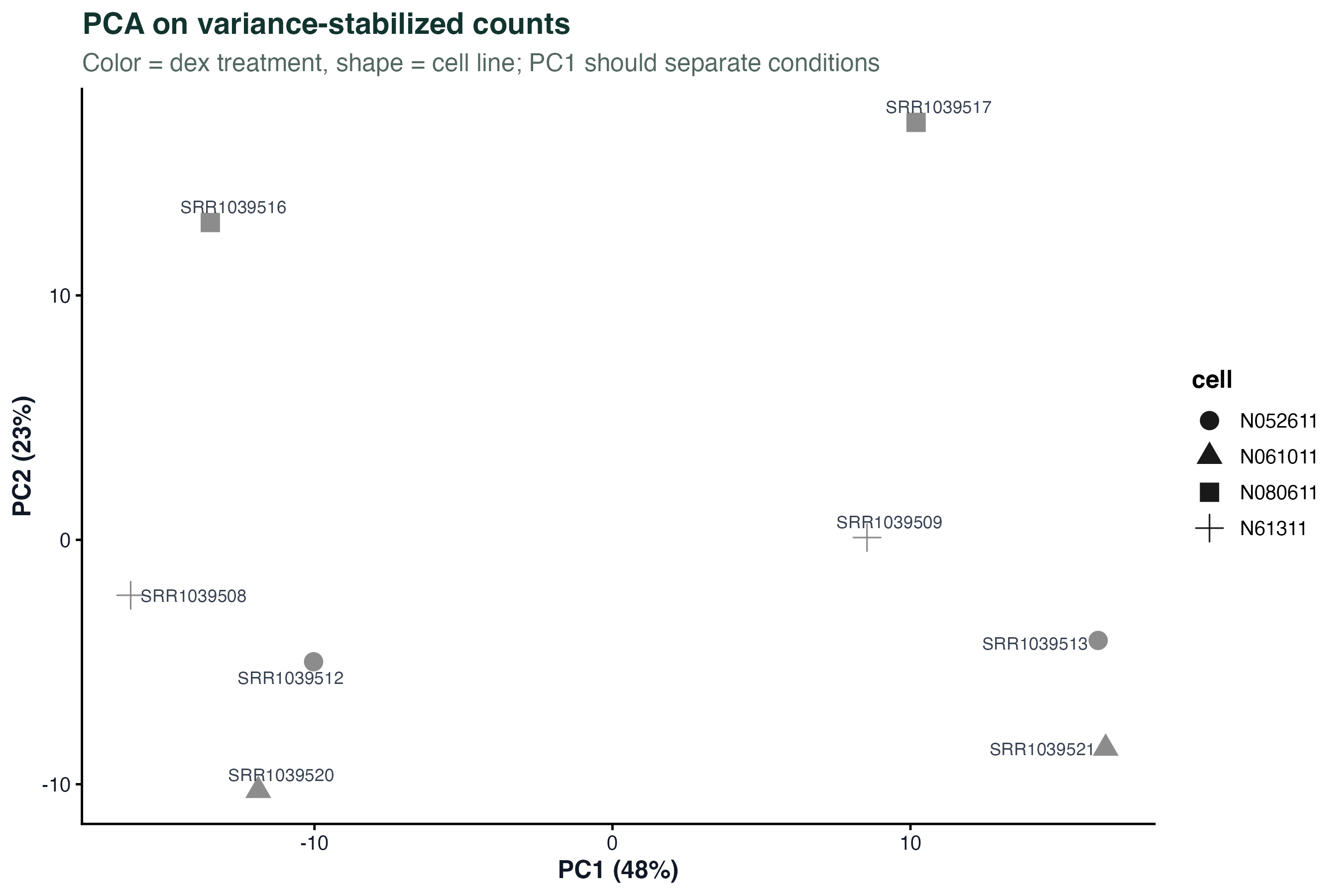
PCA Scatter
vsd <- vst(dds, blind = FALSE)
pca <- plotPCA(vsd, intgroup = "condition", returnData = TRUE)
pct <- round(100 * attr(pca, "percentVar"))
ggplot(pca, aes(PC1, PC2, color = condition)) +
  geom_point(size = 4) +
  geom_text_repel(aes(label = name), size = 3) +
  labs(x = paste0("PC1 (",pct[1],"%)"), y = paste0("PC2 (",pct[2],"%)")) +
  theme_classic()
Violin + Boxplot
ggplot(df, aes(x = condition, y = expression, fill = condition)) +
  geom_violin(width = 0.8, alpha = 0.7, color = NA) +
  geom_boxplot(width = 0.15, fill = "white", outlier.shape = NA) +
  geom_jitter(width = 0.1, size = 1.5, alpha = 0.6) +
  facet_wrap(~ gene, scales = "free_y") +
  scale_fill_manual(values = c("#475569","#dc2626"), guide = "none") +
  theme_classic()
Top Gene Counts
top_genes <- head(rownames(counts(dds, normalized = TRUE)
  [order(-rowMeans(counts(dds, normalized = TRUE))), ]), 20)
plotCounts_df <- reshape2::melt(counts(dds, normalized = TRUE)[top_genes, ])
ggplot(plotCounts_df, aes(x = Var1, y = value, fill = Var1)) +
  geom_boxplot() + coord_flip() +
  labs(x = NULL, y = "Normalized counts") +
  theme_classic() + theme(legend.position = "none")
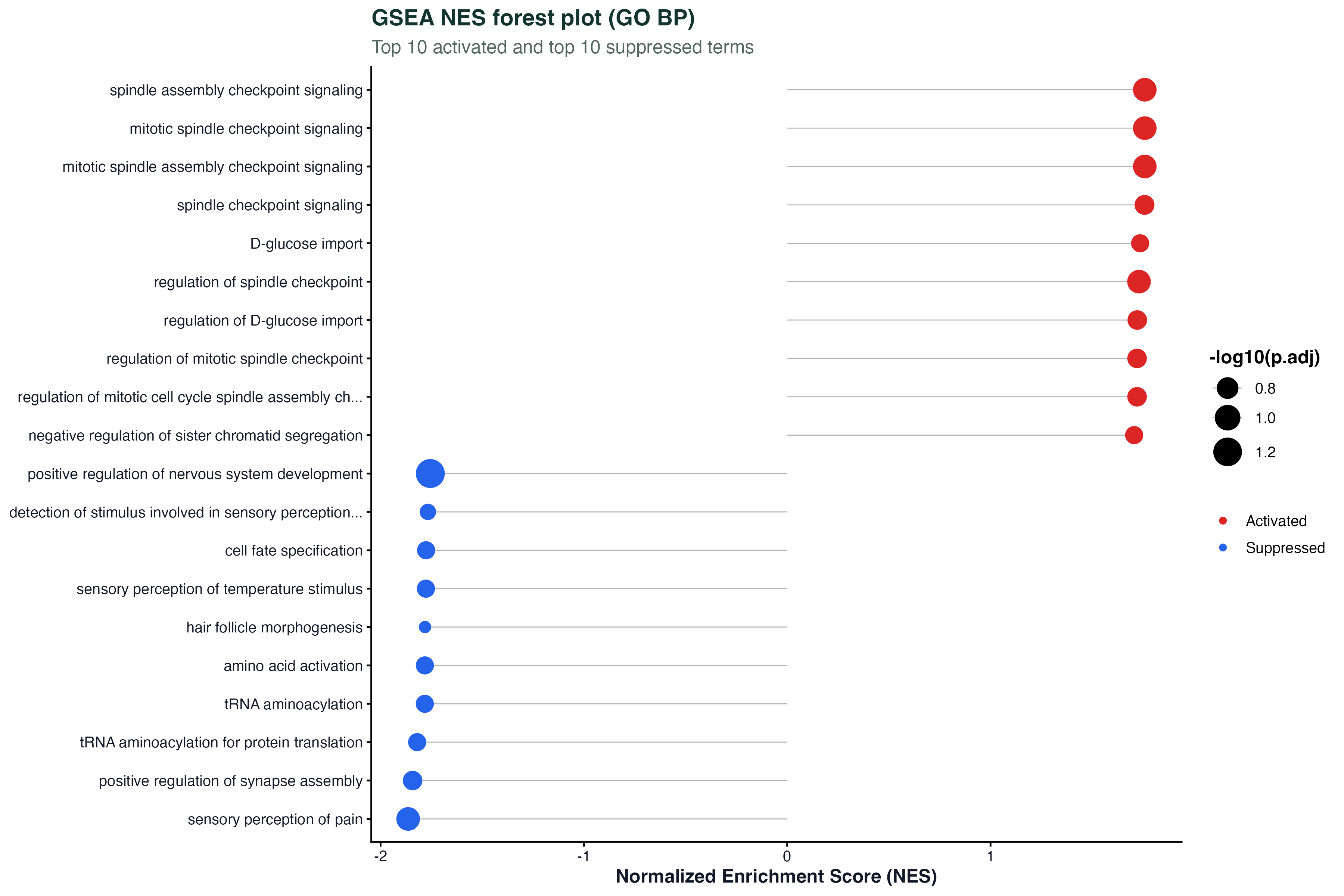
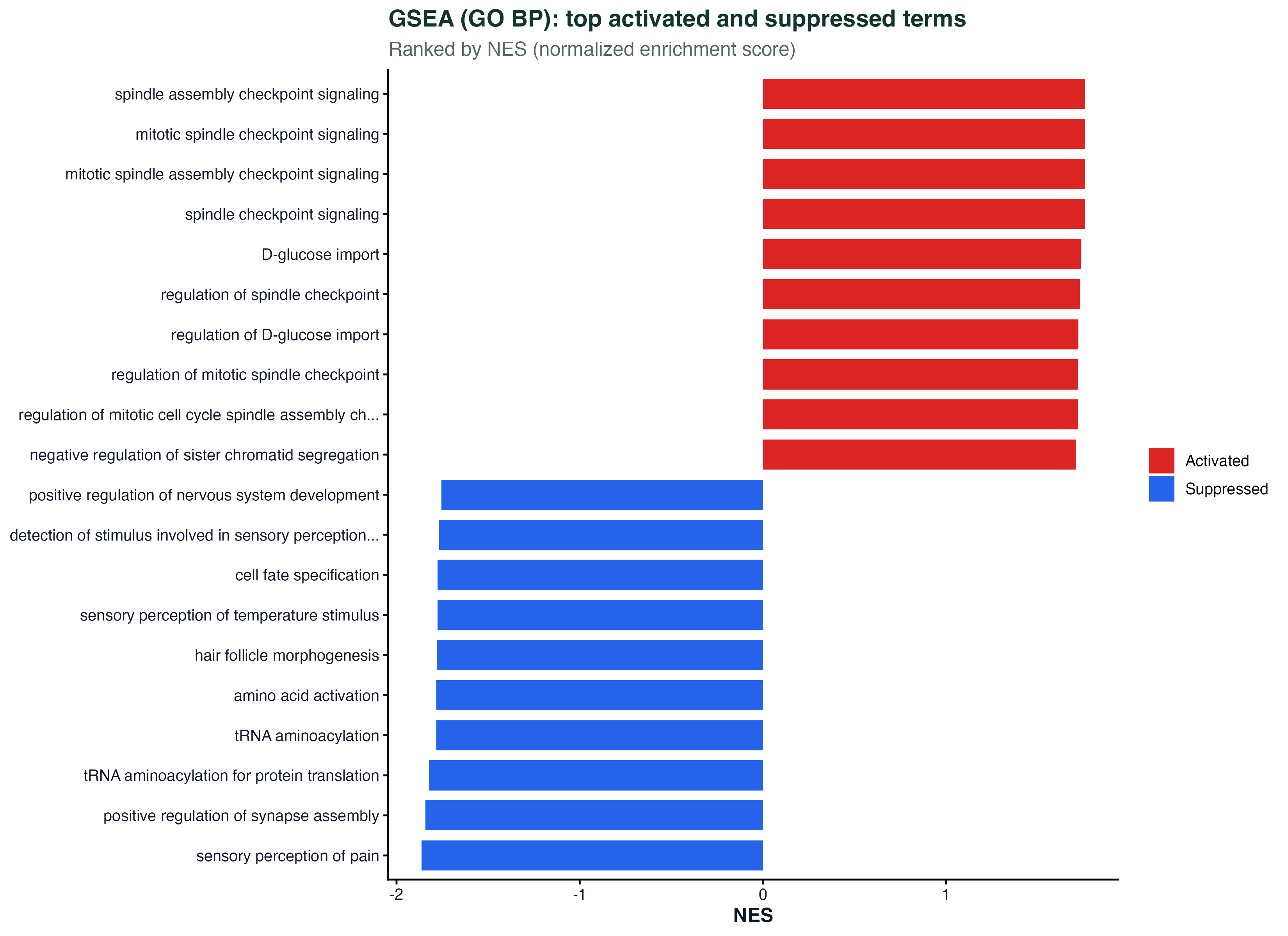
NES Forest Plot
ggplot(gsea_top, aes(x = NES, y = reorder(Description, NES))) +
  geom_point(aes(size = setSize, color = p.adjust)) +
  geom_errorbarh(aes(xmin = NES - 0.3, xmax = NES + 0.3), height = 0.2) +
  geom_vline(xintercept = 0, linetype = "dashed") +
  scale_color_gradient(low = "#dc2626", high = "#2563eb") +
  labs(x = "NES", y = NULL) + theme_classic()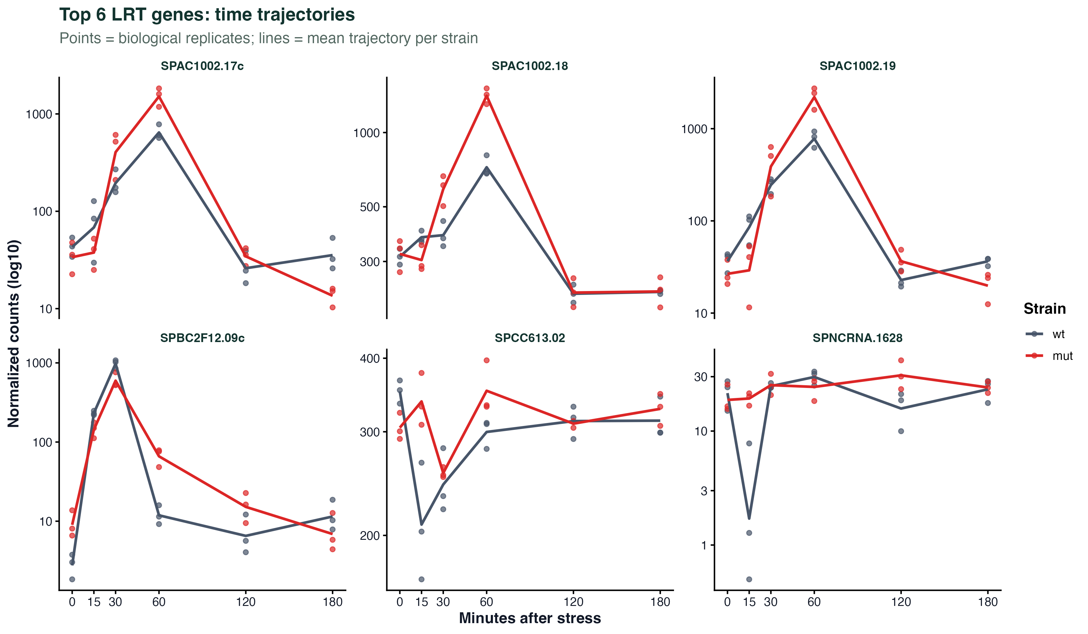
Time Trajectory
ggplot(traj_df, aes(x = time, y = expression, group = gene, color = cluster)) +
  geom_line(alpha = 0.4) +
  geom_point(size = 1.5) +
  stat_summary(aes(group = cluster), fun = mean, geom = "line", linewidth = 1.5) +
  facet_wrap(~ cluster) +
  labs(x = "Time point", y = "Scaled expression") +
  theme_classic()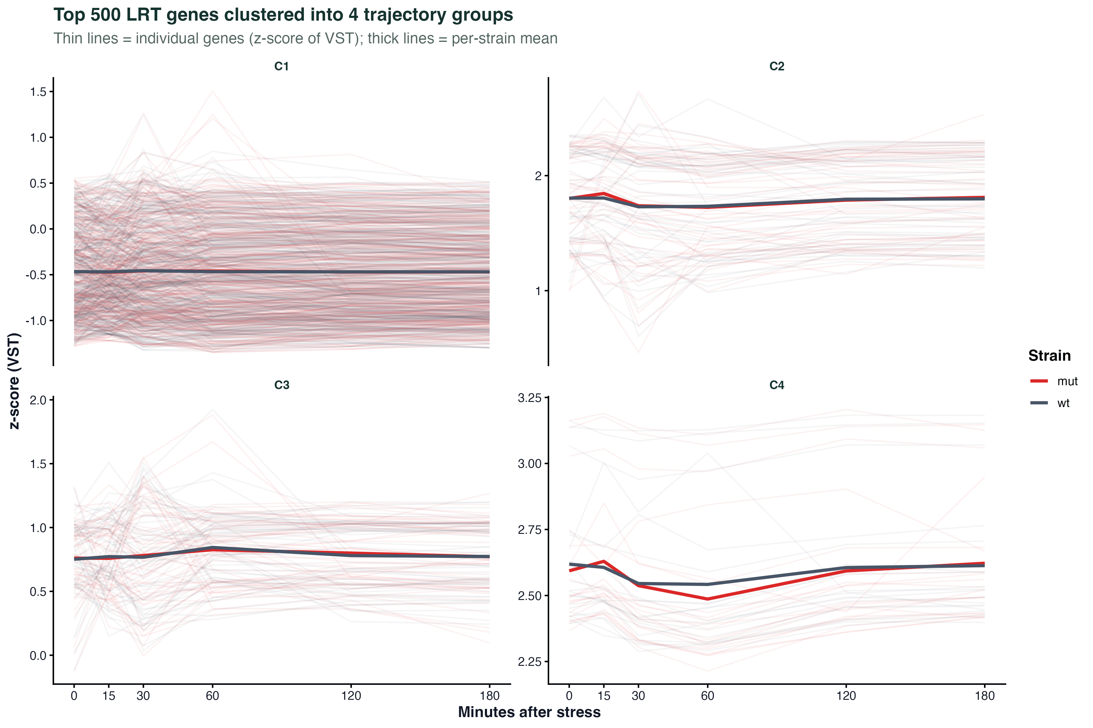
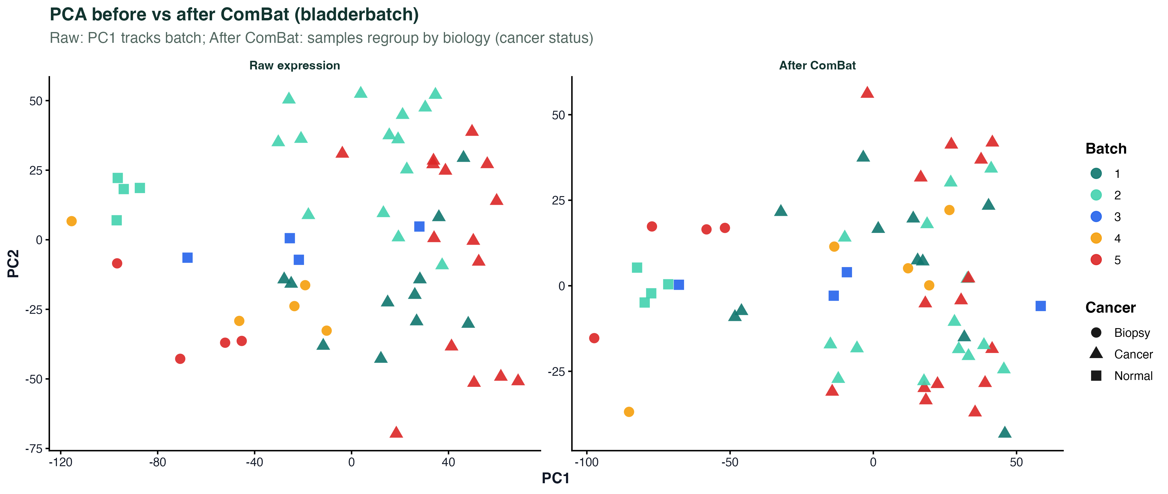
Batch Effect PCA
# Before correction
p1 <- plotPCA(vsd_before, intgroup = "batch") + ggtitle("Before ComBat")
# After correction
combat_mat <- ComBat_seq(counts, batch = batch, group = condition)
vsd_after <- vst(DESeqDataSetFromMatrix(combat_mat, colData, ~condition))
p2 <- plotPCA(vsd_after, intgroup = "condition") + ggtitle("After ComBat")
p1 + p2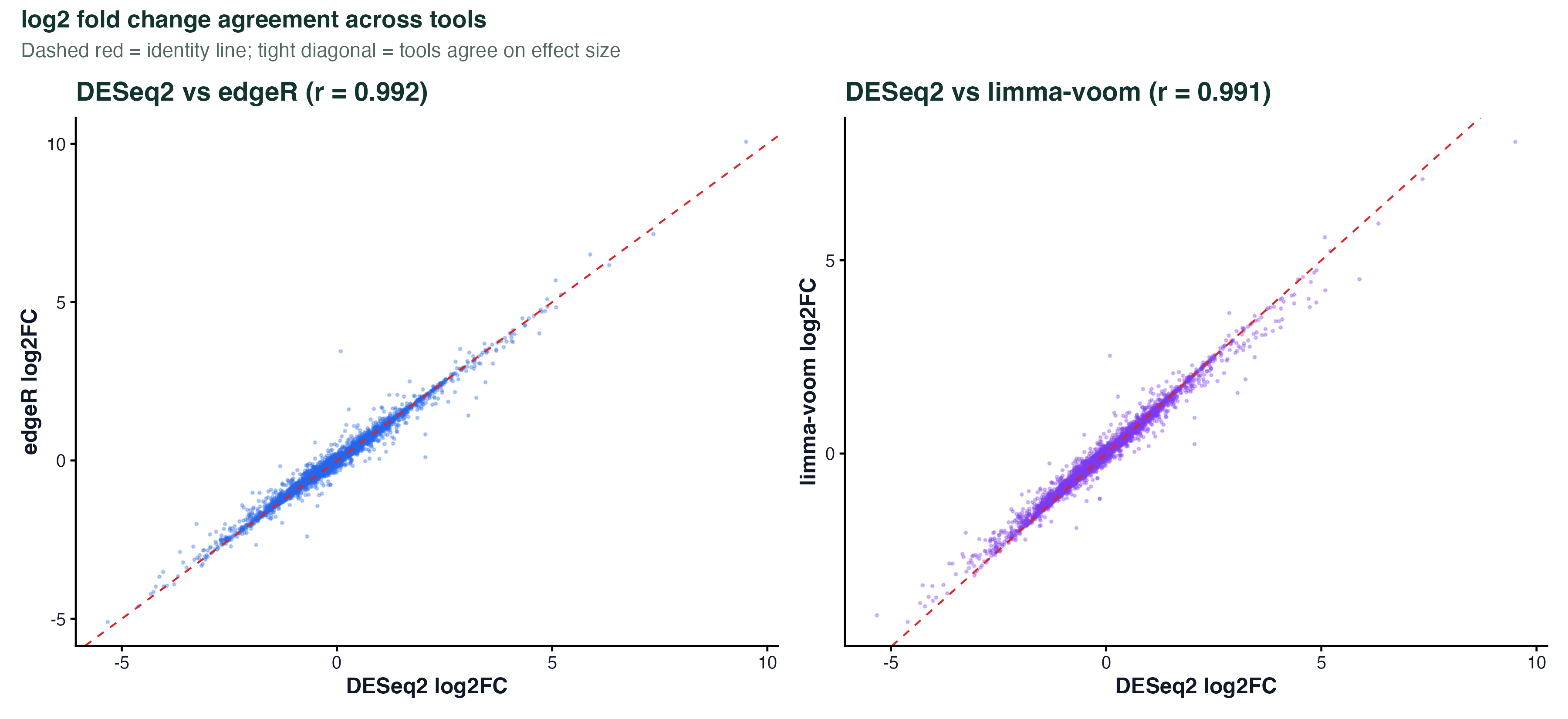
LFC Scatter
ggplot(compare_df, aes(x = lfc_deseq2, y = lfc_edger)) +
  geom_point(size = 0.8, alpha = 0.4, color = "#475569") +
  geom_abline(slope = 1, intercept = 0, linetype = "dashed", color = "red") +
  geom_smooth(method = "lm", se = FALSE, color = "#2563eb") +
  annotate("text", x = -3, y = 4, label = paste0("r = ", round(cor_val, 3))) +
  labs(x = "log2FC (DESeq2)", y = "log2FC (edgeR)") +
  theme_classic()